Influence Functions and the Hessian Estimation

• 1. Motivation
• 2. Setup
• 3. Deleting a training point
  • 3.1 Parameter change
  • 3.2 Loss change
    • 3.2.1 Self influence
  • 3.3 Output change
    • 3.3.1 Self influence
  • 3.4 Special Cases
    • 3.4.1 Regression
    • 3.4.2 Classification
    • 3.4.3 Linear models
      • Linear regression
      • Logistic regression
• 4. Perturbing a training input
• 5. Hessian estimation
  • 5.1 Direct method
  • 5.2 Conjugate gradient
  • 5.3 Stochastic estimation
  • 5.4 Outer-product approximation
  • 5.5 Diagonal approximation
  • 5.6 Validation
• Reference

1. Motivation

Understanding how sensitive a model is to its training data is both important and challenging. To assess the impact of a training point on a prediction, we often ask the following counterfactual question:

What would happen if this training point were removed, or if its value were changed slightly?

This question is central to many practical concerns in machine learning, including data quality, privacy, and security. For example, it can help us identify mislabeled or biased training examples, understand whether a model relies on sensitive or private information, and analyze how vulnerable the model is to malicious manipulation of the training data.

A straightforward way to answer such questions is to delete or perturb a training point and retrain the model. However, this is often computationally prohibitive, especially for modern large-scale models. To address this challenge, we turn to influence functions, a classical tool from robust statistics that provides a local approximation of how small changes in the training data affect the learned model. In this blog, we review influence functions for deleting and perturbing a training point, and analyze how these changes affect the model parameters, the loss, and the output. We also discuss Hessian estimation, which plays a central role in influence-function-based analysis, and explain how it can be computed efficiently in practice.

2. Setup

Consider a classification setting where the goal is to map an instance \(\mathbf{x} \in \mathcal{X}\) to a label \(y \in \mathcal{Y}=[K]\). We are given training points \(\mathbf{z}_1,\cdots,\mathbf{z}_n\), where \(\mathbf{z}_i=(\mathbf{x}_i,y_i)\in \mathcal{X}\times \mathcal{Y}\). For a point \(\mathbf{z}\) and parameters \(\boldsymbol{\theta}\), let \(\ell(\mathbf{z},\boldsymbol{\theta})\) be the loss, and let \(\frac{1}{n}\sum_{i=1}^n \ell(\mathbf{z}_i, \boldsymbol{\theta})\) be the empirical risk. The empirical minimizer is given by

Assume that the empirical risk is twice-differentiable and strictly convex in \(\boldsymbol{\theta}\).

3. Deleting a training point

We ask the following counterfactual question:

What would happen if this training point were removed?`

3.1 Parameter change

Formally, this change is \(\hat{\boldsymbol{\theta}}_{-\mathbf{z}} - \hat{\boldsymbol{\theta}}\), where

Influence functions gives us an efficient approximation without retraining the model for removing \(\mathbf{z}\). The idea is to compute the parameter change if \(\mathbf{z}\) were weighted by some small \(\epsilon\), giving us new parameters

Let \(\Delta_{\boldsymbol{\theta}}(\mathbf{z}) \overset{\text{def}}{=} \frac{d \hat{\boldsymbol{\theta}}_{\epsilon,\mathbf{z}} }{d \epsilon}\bigg|_{\epsilon = 0}\) be the infinitesimal parameter change. Using first-order Taylor expansion, we have

The infinitesimal parameter change is given by:

where \(H_{\hat{\boldsymbol{\theta}}}=\frac1n\sum_{i=1}^n \nabla^2 \ell(\mathbf{z}_i, \hat{\boldsymbol{\theta}})\) is the Hessian and is positive definite (PD) by assumption.

The parameter change due to removing \(\mathbf{z}\) can be linearly approximated as:

The learned parameter \(\hat{\boldsymbol{\theta}}\) can be viewed as a local equilibrium determined by all training samples. Each point contributes a gradient, which indicates the direction in which it tends to pull the model in order to reduce its own loss. Removing one sample \(\mathbf z\) removes this pull, and the optimum shifts slightly as a result.

The gradient \(\nabla_{\boldsymbol{\theta}}\ell(\mathbf z,\hat{\boldsymbol{\theta}})\) captures the individual effect of sample \(\mathbf z\), while the inverse Hessian \(H_{\hat{\boldsymbol{\theta}}}^{-1}\) adjusts this effect according to the local curvature of the loss landscape. Directions with high curvature are harder to move, whereas flatter directions are more sensitive. Therefore, this formula says that the parameter change caused by removing one point is approximately its own gradient contribution, scaled by \(1/n\) and corrected by the local geometry.

3.2 Loss change

Next, we apply the chain rule to measure how deleting \(\mathbf{z}\) changes the loss function at a test point \(\mathbf{z}_\mathsf{test}\). Let

be the infinitesimal loss change. Using first-order Taylor expansion, the loss change has the expression:

The infinitesimal loss change is given by:

The loss change due to removing \(\mathbf{z}\) can be linearly approximated as:

It compares the direction in which the test point would like to move the parameters with the direction contributed by the training point, after correcting for the local geometry of the loss landscape.

Let \(S(\mathbf z,\mathbf z_{\mathsf{test}}) := \nabla_{\boldsymbol{\theta}}\ell(\mathbf{z}_{\mathsf{test}},\hat{\boldsymbol{\theta}})^\top H^{-1}_{\hat{\boldsymbol{\theta}}} \nabla_{\boldsymbol{\theta}}\ell(\mathbf{z},\hat{\boldsymbol{\theta}}).\) Then:

• If \(S(\mathbf z,\mathbf z_{\mathsf{test}}) > 0\), then \(\ell(\mathbf{z}_{\mathsf{test}}, \hat{\boldsymbol{\theta}}_{-\mathbf{z}}) - \ell(\mathbf{z}_{\mathsf{test}}, \hat{\boldsymbol{\theta}}) > 0,\) so removing \(\mathbf z\) increases the test loss: \(\mathbf z\) is helpful for \(\mathbf z_{\mathsf{test}}\).

• If \(S(\mathbf z,\mathbf z_{\mathsf{test}}) < 0\), then \(\ell(\mathbf{z}_{\mathsf{test}}, \hat{\boldsymbol{\theta}}_{-\mathbf{z}}) - \ell(\mathbf{z}_{\mathsf{test}}, \hat{\boldsymbol{\theta}}) < 0,\) so removing \(\mathbf z\) decreases the test loss: \(\mathbf z\) is harmful for \(\mathbf z_{\mathsf{test}}\).

• If \(S(\mathbf z,\mathbf z_{\mathsf{test}}) \approx 0\), then removing \(\mathbf z\) has little first-order effect on the prediction at \(\mathbf z_{\mathsf{test}}\).

3.2.1 Self influence

When \(\mathbf z_{\mathsf{test}}=\mathbf z\), the influence reduces to the self-influence

Under the local convexity assumption, \(H_{\hat{\boldsymbol\theta}}^{-1}\) is positive definite, so this quantity is nonnegative. Thus, removing a training point typically increases its own loss. Moreover, the magnitude is not determined only by the gradient norm, but also by the local curvature: directions with smaller curvature are amplified by \(H^{-1}\), while directions with larger curvature are suppressed.

3.3 Output change

Next, we study how deleting a training point \(\mathbf{z}\) changes the model output at a test point \(\mathbf{z}_\mathsf{test}\). Let \(f(\mathbf{x}, \boldsymbol{\theta})\) denote the model output. For simplicity, we first consider the scalar-output case, where \(f(\mathbf{x}, \boldsymbol{\theta}) \in \mathbb{R}\). Let

be the infinitesimal output change. Using a first-order Taylor expansion, the output change due to removing \(\mathbf z\) can be approximated as

The infinitesimal output change is given by

Therefore, the output change due to removing \(\mathbf z\) can be linearly approximated as

It tells us how much the prediction at \(\mathbf x_{\mathsf{test}}\) changes when the contribution of training point \(\mathbf z\) is removed. The quantity \(\nabla_{\boldsymbol\theta} f(\mathbf x_{\mathsf{test}},\hat{\boldsymbol\theta})^\top H_{\hat{\boldsymbol\theta}}^{-1} \nabla_{\boldsymbol\theta}\ell(\mathbf z,\hat{\boldsymbol\theta})\) can be viewed as a curvature-adjusted alignment between the training-point gradient and the sensitivity of the test output.

3.3.1 Self influence

When \(\mathbf z_{\mathsf{test}}=\mathbf z\), the formula reduces to

This quantity measures how much the model’s own prediction on a training point changes after that point is removed from the training set. Unlike the self-loss influence, its sign is not necessarily fixed: depending on the local geometry and on the relation between \(\nabla_{\boldsymbol\theta} f(\mathbf x,\hat{\boldsymbol\theta})\) and \(\nabla_{\boldsymbol\theta}\ell(\mathbf z,\hat{\boldsymbol\theta}),\) the output may either increase or decrease.

3.4 Special Cases

The general influence formulas apply to a broad class of differentiable models. However, in several important settings, they admit simpler and more interpretable forms.

3.4.1 Regression

In regression, the model output is typically scalar, \(f(\mathbf{x},\boldsymbol{\theta})\in \mathbb{R}\). A common choice is the squared loss

In this case,

so the influence is proportional to the prediction error \(\left(f(\mathbf{x},\hat{\boldsymbol{\theta}})-y\right)\).

3.4.2 Classification

Consider the binary classification case, where the model produces a scalar logit \(f(\mathbf{x},\boldsymbol{\theta}) \in \mathbb{R}\). Under the cross-entropy loss,

the derivative of the loss with respect to the output is

Therefore, by the chain rule,

3.4.3 Linear models

For linear models, the influence formulas become particularly explicit because the Hessian can be written in closed form. Consider a linear predictor

Linear regression

For squared-loss linear regression, \(\ell(\mathbf z,\boldsymbol\theta)=\frac12(\boldsymbol\theta^\top\mathbf x-y)^2.\) Then

Hence (recall that \(H_{\hat{\boldsymbol{\theta}}} = \frac{1}{n}\sum_{i=1}^n \nabla_{\boldsymbol{\theta}}^2 \ell(\mathbf z_i,\hat{\boldsymbol{\theta}})\)),

The loss change and the output change can be analyzed analogously.

Logistic regression

Under the binary cross-entropy loss,

and

Therefore,

The loss change and the output change can be analyzed analogously.

4. Perturbing a training input

We ask the following counterfactual question:

What would happen if this training input were modified?`

For a training point \(\mathbf{z}=(\mathbf{x},y)\), define \(\mathbf{z}_{\boldsymbol{\delta}} \overset{\text{def}}{=} (\mathbf{x}+\boldsymbol{\delta},y).\) Consider the perturbation \(\mathbf{z} \rightarrow \mathbf{z}_\boldsymbol{\delta}\), and let \(\hat{\boldsymbol{\theta}}_{\mathbf{z}_\boldsymbol{\delta},-\mathbf{z}}\) be the empirical risk minimizer on the training points with \(\mathbf{z}_\boldsymbol{\delta}\) in place of \(\mathbf{z}\). To approximate its effects, define the parameters resulting from moving \(\epsilon\) mass from \(\mathbf{z}\) onto \(\mathbf{z}_\boldsymbol{\delta}\):

An analogous computation yields:

As before, we can make the linear approximation

giving us a closed-form estimate of the effect of \(\mathbf{z} \rightarrow \mathbf{z}_\boldsymbol{\delta}\) on the model. Analogous equations also apply for changes in \(y\). While influence functions might appear to only work for infinitesi- mal (therefore continuous) perturbations, it is important to note that this approximation holds for arbitrary \(\boldsymbol{\delta}\): the \(\epsilon\)-upweighting scheme allows us to smoothly interpolate between \(\mathbf{z}\) and \(\mathbf{z}_\boldsymbol{\theta}\). This is particularly useful for working with discrete data (e.g., in NLP) or with discrete label changes.

Assume that the input domain \(\mathcal{X}\subseteq\mathbb{R}^d\), the parameter space \(\Theta\subseteq\mathbb{R}^p\), and the loss function \(\ell\) is differentiable with respect to both \(\boldsymbol{\theta}\) and \(\mathbf{x}\). If \(\boldsymbol{\delta}\) is small, then

where \(\nabla_{\mathbf{x}}\nabla_{\boldsymbol{\theta}}\ell(\mathbf{z},\hat{\boldsymbol{\theta}}) \in \mathbb{R}^{p\times d}.\) Substituting this into the perturbed parameter-change formula gives

Therefore,

Differentiating with respect to \(\boldsymbol{\delta}\) and applying the chain rule, we define the infinitesimal loss change due to perturbing the training input as \(\Delta_\ell(\mathbf{z},\mathbf{z}_{\mathsf{test}}) \overset{\text{def}}{=} \nabla_{\boldsymbol{\delta}} \ell(\mathbf{z}_{\mathsf{test}},\hat{\boldsymbol{\theta}}_{\mathbf{z}_{\boldsymbol{\delta}},-\mathbf{z}}) \bigg|_{\boldsymbol{\delta}=0}.\) It is given by

Hence, the loss change due to perturbing the training input can be linearly approximated as

5. Hessian estimation

Except in linear models, where closed-form expressions are available, a practical bottleneck in influence functions is the computation of the Hessian \(H_{\hat{\boldsymbol{\theta}}}\), and especially its inverse. In this section, we first review the direct method (exact computation), and then discuss several efficient estimation and approximation methods, including conjugate gradients, stochastic estimation, diagonal approximation, and outer-product approximation.

5.1 Direct method

The most direct approach is to first compute the full Hessian matrix \(H_{\hat{\boldsymbol{\theta}}} = \frac1n\sum_{i=1}^n \nabla_{\boldsymbol{\theta}}^2 \ell(\mathbf z_i,\hat{\boldsymbol{\theta}})\) and then compute its inverse \(H_{\hat{\boldsymbol{\theta}}}^{-1}\). However, if the model has \(p\) parameters, forming the Hessian costs \(O(np^2)\) operations and storing it requires \(O(p^2)\) memory, while matrix inversion costs an additional \(O(p^3)\). This quickly becomes prohibitive for modern models.

In PyTorch, this direct method can be implemented by defining the empirical risk as a function of the parameter vector and then calling torch.autograd.functional.hessian to obtain the full Hessian matrix. Once the Hessian is formed, one can compute its inverse explicitly. E.g.

# theta: parameter vector of shape (p,)
# loss_fn: empirical risk as a scalar function of theta
H = torch.autograd.functional.hessian(loss_fn, theta)
H_inv = torch.linalg.inv(H)

5.2 Conjugate gradient

The first technique is to avoid explict inversion of the Hessian matrix, which transforms it into an optimization problem. Since \(H_\hat{\boldsymbol{\theta}} \succ 0\) by assumption,

We can solve this with conjugate gradient approaches that only require the evaluation of \(H_\hat{\boldsymbol \theta} \mathbf{t}\), which takes \(O(np)\), without explicitly forming \(H_\hat{\boldsymbol \theta}\). While an exact solution takes \(p\) iterations, in practice we can get a good approximation with fewer iterations

5.3 Stochastic estimation

With large datasets, standard conjugate gradient can be slow; each iteration still goes through all \(n\) training points. We use a method developed by Agarwal et al. (2017) to get an estimator that only samples a single pointper iteration, which results in significant speedups. Dropping the \(\hat{\boldsymbol{\theta}}\) subscript for clarity, let us first introduce the approximate matrix inversion based on truncated Neumann-series. Suppose \(H\) is invertible and \(\|H\| \leq 1\) (if this is not true, we can scale the loss down without affecting the parameters), we have

Let \(H_j^{-1} \overset{\text{def}}{=} \sum_{i=0}^j(1-H)^{i}\), the first \(j\) terms in the expansion of \(H^{-1}\). Rewrite this recursively as

\(H_j^{-1} \rightarrow H^{-1}\) as \(j \rightarrow \infty\). The key is that at each iteration, we can substi- tute the full H with a draw from any unbiased (and faster-to-compute) estimator of \(H\) to form \(\tilde{H}_j\). Since \(\mathbb{E}[\tilde{H}_j^{-1}]=H_j^{-1}\), we still have \(\mathbb{E}[\tilde{H}_j^{-1}]\rightarrow H^{-1}\).

In particular, for any training point \(\mathbf z_i\), we can use \(\nabla_{\boldsymbol{\theta}}^2 \ell(\mathbf z_i,\hat{\boldsymbol{\theta}})\) as an unbiased estimator of \(H_{\hat{\boldsymbol{\theta}}}.\) This leads to the following stochastic procedure: uniformly sample \(t\) points \(\mathbf z_{s_1},\ldots,\mathbf z_{s_t}\) from the training data, initialize \(\tilde H_0^{-1}\mathbf v=\mathbf v,\) and recursively compute

We then take \(\tilde H_t^{-1}\mathbf v\) as the final unbiased estimate of \(H_{\hat{\boldsymbol{\theta}}}^{-1}\mathbf v.\) In practice, we choose \(t\) large enough so that the recursion stabilizes, and to reduce variance, we repeat this procedure \(r\) times and average the results.

5.4 Outer-product approximation

Another common surrogate is to replace the Hessian by an outer-product matrix:

This is related to empirical Fisher or Gauss-Newton style approximations. Its appeal is that it is always positive semidefinite and often easier to estimate. However, it comes with two caveats. First, it is not the true Hessian in general. Second, it may be low-rank or severely ill-conditioned, especially in overparameterized models, so its inverse may not exist or may be numerically unstable. In practice, one usually adds damping,

5.5 Diagonal approximation

Previous methods (direct method, conjugate gradient and stochastic estimation) produce unbiased estimation of Hessian (or related computation). A much cheaper approximation is to retain only the diagonal of the Hessian or inverse Hessian:

This ignores cross-parameter interactions, so it is clearly less faithful than the full matrix. However, it is simple, memory-efficient, and often good enough when one only needs a rough ranking of influential points. In practice, we can further simplify the computation by restricting the estimation it to the last layer, reducing complexity from quadratic to essentially linear in the number of parameters.

5.6 Validation

Here, we empirically compare the above-mentioned Hessian estimation methods on 10-class MNIST using a logistic regression model. We train the model with L-BFGS and \(L_2\) regularization of 0.01, with \(n=55{,}000\) training samples and \(p=7{,}840\) parameters. We arbitrarily select a misclassified test point \(\mathbf{z}_{\mathsf{test}}\). Among all training points, we take the 500 points \(\mathbf z\) with the largest values of \(\Delta_\ell(\mathbf z,\mathbf z_{\mathsf{test}})\), and for each of them we compare the estimated value of \(-\frac1n\Delta_\ell(\mathbf z,\mathbf z_{\mathsf{test}})\) under the different estimation methods, with the true change in test loss obtained by removing that point and retraining the model.

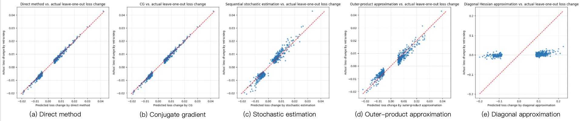
The direct method and conjugate gradient (CG) align almost perfectly with the actual leave-one-out retraining results, showing that influence functions can be highly accurate when the Hessian inverse is computed reliably. Stochastic estimation and outer-product approximation still capture the overall trend, but with noticeably larger variance. In contrast, the diagonal approximation performs substantially worse, indicating that the off-diagonal structure of the Hessian is important even in this simple logistic-regression setting. Overall, the experiments reveal a clear trade-off between efficiency and accuracy: direct inversion and CG are the most accurate, stochastic and outer-product methods are reasonable approximations, and the diagonal approximation is too crude for precise prediction.

Reference

1. Pang Wei Koh and Percy Liang. Understanding black-box predictions via influence functions. In ICML 2017.
2. Nickl et al. The memory perturbation equation: understanding model’s sensitivity to data. In NeurIPS 2023.
3. Agarwal et al. Second order stochastic optimization in linear time. JMLR 2017.